Decidability and Definability

January 15, 2019January 15, 2019 ~ Athar ~ Leave a comment

This post is an extension of the previous one; I want to address Tarski’s Undefinability Theorem using computability-theoretic methods. Continue reading →

Arithmetic, Self-Reference and Truth

January 13, 2019January 13, 2019 ~ Athar ~ Leave a comment

There is a remarkable theorem in mathematical logic that “Truth is not definable”. This is known as Tarski’s Undefinability Theorem. This result (along with Gödel’s Incompleteness Theorems) has fascinated me ever since I learned about it. This theorem (in a sense) shows us the limits of the ability to study truth within a given formal system. Continue reading →

Ramsey’s Theorem and Ultrafilters

April 7, 2018 ~ Athar ~ Leave a comment

In this post, I will go through a proof of one of my favorite results in combinatorics using a technique that is not necessarily well known outside of logic.

Ramsey’s Theorem

There are many ways to describe (Infinite) Ramsey’s Theorem. One description uses graph theory. A graph is a set of vertices (nodes) and edges (connections between the nodes). A clique in a graph is a subset X of the set of vertices such that all vertices in X have edges between them. An anti-clique is a subset X of the set of vertices such that no two vertices in X have edges between them.

Theorem: Every infinite graph has an infinite clique or an infinite anti-clique.

We can formalize Ramsey’s Theorem in another way. A two-coloring of a set X is a function $f : X \to \{ 0, 1 \}$ ; in other words, a partition of X into two sets (the elements 0 and 1 are the “colors”, often representing blue and red). GIven a set X, the set $[X]^2$ is the set of pairs of elements of X. For example, the set $[\mathbb{N}]^2$ is the set of (unordered) pairs of natural numbers, e.g., it’s the set {0, 1}, {0, 2}, {1, 2}, {0, 3}, etc.

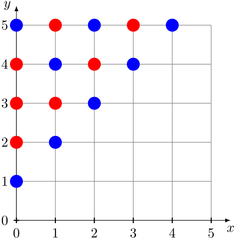Theorem (Ramsey’s Theorem for Pairs): If f is a two-coloring of $[\mathbb{N}]^2$ , there is an infinite set H such that all pairs of elements of H get the same color.

These two theorems are equivalent: given a two-coloring of the set of pairs of natural numbers, you can form an infinite graph by letting the set of vertices just be $\mathbb{N}$ , and by putting an edge between numbers n and m if and only if the color $f(n, m) = 1$ . You can also go the other way: given a graph, you can form a two-coloring of the set of pairs of vertices of the graph in a canonical way.

This second statement, while more difficult to parse, is the one we will focus on for this post.

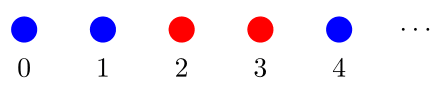
First, let’s prove an easier statement: if $f$ is a two-coloring of $\mathbb{N}$ , there is an infinite set X such that every element of X gets the same color. (This would be referred to as “Ramsey’s Theorem for Singletons”.)

ramsey-1 — A two-coloring of $\mathbb{N}$

This result is fairly easy to prove: let 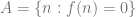$A = \{ n : f(n) = 0 \}$ and $B = \{ n : f(n) = 1 \}$ . One of these two sets must be infinite, and every element of A gets color 0 (blue), while every element of B gets 1 (red).

If we try to generalize this proof to Ramsey’s Theorem for Pairs, we can look at the sets $A = \{ \{ x, y \} : f(x, y) = 0 \}$ and $B = \{ \{ x, y \} : f(x, y) = 1 \}$ ; clearly one of these is infinite. But these sets are sets of pairs, and Ramsey’s Theorem states that there is an infinite set of numbers where all the pairs of numbers get the same color (in graph-theoretic terms, it’s easy to find an infinite set of edges or non-edges in an infinite graph; we want an infinite set of vertices which are either all mutually connected or mutually disconnected).

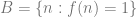
The reason Ramsey’s Theorem for Singletons is easy to prove is because we know the color of each number; we know $f(0), f(1),$ etc. But if we are coloring pairs, then perhaps $f(0, 1) = 0, f(0, 2) = 1, f(0, 3) = 0,$ . In other words, the color of 0 might be blue infinitely often, and it might be red infinitely often. We need a way to decide the color of each natural number “on average”. That is, if we could say, given a natural number n, “for most numbers m, $f(n, m) = 0$ “, or, “for most numbers m, $f(n, m) = 1$ “.

Of course, it is not obvious that it is possible to make such a claim for each number n. Sometimes it’s clear: if, for example, the color “stabilizes”; ie, maybe $f(0, 1) = 0, f(0, 2) = 1, f(0, 3) = 0,$ and for all $n > 3$ , $f(0, n) = 1$ . In that case, it is clear that the color of 0 is “usually” 1. But perhaps the color does not stabilize: maybe there are infinitely many numbers m such that $f(0, m) = 0$ and infinitely many n such that $f(0, n) = 1$ . So in that case, how would you decide what the color of 0 is on average?

Ultrafilters: “averaging” over infinity

This idea of averaging over an infinite set can be studied formally with the concept of an ultrafilter. An ultrafilter is a way of choosing which sets are “large”.

Definition: A filter on the natural numbers is a family of sets $\mathcal{F}$ with the following properties:

for any sets A and B, if $A \in \mathcal{F}$ and $A \subseteq B \subseteq \mathbb{N}$ , then $B \in \mathcal{F}$
for any sets $A, B \in \mathcal{F}$ , the intersection $A \cap B \in \mathcal{F}$
$\emptyset \not \in \mathcal{F}$ .

An ultrafilter is a filter $\mathcal{U}$ with the additional property that for all $X \subseteq \mathbb{N}$ , either $X \in \mathcal{U}$ or $\mathbb{N} \setminus X \in \mathcal{U}$ .

Again, the idea is that the sets in an ultrafilter are considered “large”. Each of these properties represents some “largeness” principle. If a set is large, any set that contains it should also be large; if two sets are large, their intersection is large; the empty set is not large; and if a set is not large, the complement of it should be large. We say that a property “almost always” happens if it happens on a large set, and it “almost never” happens if it happens on a set which is not large.

There are some easy examples of ultrafilters: take any number n, and let $\mathcal{U}_n = \{ A \subseteq \mathbb{N} : n \in A \}$ . It’s not hard to verify that all the properties are satisfied. Ultrafilters like these (the ones generated in some sense by a single number) are called principal. Non-principal ultrafilters are harder to construct, but given some amount of set theory it is possible to show that they also exist. Non-principal ultrafilters have a crucial property: they contain no finite sets. That means that if A is the complement of a finite set (“cofinite”), then A is in every non-principal ultrafilter.

Proof of Ramsey’s Theorem

Let $f : [\mathbb{N}]^2 -> \{0, 1\}$ . Let $\mathcal{U}$ be a non-principal ultrafilter. We use the ultrafilter $\mathcal{U}$ to assign colors to each number as follows: $g : \mathbb{N} \to \{ 0, 1 \}$ is defined as $g(n) = 0$ if and only if $\{ x : f(n, x) = 0 \} \in \mathcal{U}$ , and $g(n) = 1$ otherwise. Notice that $g(n) = 1$ if and only if $\{ x : f(n, x) = 1 \} \in \mathcal{U}$ . In other words, think of $f$ as assigning an infinite sequence of colors to $n$ . Then, using the ultrafilter, we pick out the color of $n$ “almost always”, and call that color $g(n)$ .

We will define a sequence by induction. Let $a_0 = 0$ . Given $a_0, \ldots, a_n$ , let $a_{n+1}$ be the least $a > a_n$ such that $f(a_i, a) = g(a_i)$ for each $i \leq n$ . We must show that such an $a$ exists. The idea here is that the function $g$ assigns the “correct” color according to the ultrafilter; that is, for each $i$ , the set of those $x$ such that $f(a_i, x) = g(a_i)$ is large. Since the intersection of finitely many large sets is also large, the set $X = \{ x : f(a_i, x) = g(a_i)$ for all $i \leq n \}$ is large. Furthermore, in a non-principal ultrafilter, large sets are always infinite, so there must be an $a \in X$ greater than $a_n$ .

Let $Y = \{ a_n : n \in \mathbb{N} \}$ , $B = \{ a \in Y: g(a) = 0 \}$ and $R = \{ a \in Y : g(a) = 1 \}$ . Clearly $Y$ is infinite, so one of $B$ or $R$ is infinite. Further, for all $x < y \in B, f(x, y) = 0$ and for all $x < y \in R, f(x, y) = 1$ , so one of $B$ or $R$ is the infinite set required by the statement of Ramsey’s Theorem.

Other applications of ultrafilters

Ultrafilters have applications all throughout mathematics, including in model theory, social choice, and non-standard analysis. I hope to explore non-standard analysis, in particular, in a future post, where I will discuss ideas like formalizing the notion of a limit using infinitesimals (instead of using epsilons and deltas).

Classifying Enayat Models of Peano Arithmetic – ASL Winter Meeting (JMM)

January 10, 2018January 15, 2018 ~ Athar ~ Leave a comment

Update (1/15): See slides here.

I will be contributing a session at the 2018 ASL Winter Meeting at the Joint Mathematics Meetings on Saturday, January 13. This talk is based on a recent paper of mine which can be found on the arxiv here.

Abstract: Simpson used arithmetic forcing to show that every countable model $\mathcal{M} \models \mathrm{PA}$ has an undefinable, inductive subset $X \subseteq M$ such that the expansion $(\mathcal{M}, X)$ is pointwise definable. Enayat later showed that there are many models with the property that every expansion upon adding a predicate for an undefinable class is pointwise definable. We refer to models with this property as Enayat models. That is, a model $\mathcal{M} \models \mathrm{PA}$ is Enayat if for each undefinable class $X \subseteq M$ , the expansion $(\mathcal{M}, X)$ is pointwise definable. In this talk we show that a model is Enayat if it is countable, has no proper cofinal submodels and is a conservative extension of each of its elementary cuts.

What is Peano Arithmetic?

June 19, 2017June 19, 2017 ~ Athar ~ Leave a comment

I recently defended my dissertation and I have had a number of non-mathematician friends and family asking me to try to explain what it is I study. In a nutshell, I study models of Peano Arithmetic and their elementary extensions. This post is meant to give an introduction to Peano Arithmetic and in a later post I will go into more details about the problems I have been working on.

Peano Axioms

My research is primarily in the first-order theory of Peano Arithmetic (PA). “First-order” refers to first-order logic, which I like to think of as providing a framework for formalizing mathematics. In first-order logic, we can express statements like “multiplication distributes over addition” as “ $\forall a \forall b \forall c (a \times (b + c) = (a \times b) + (a \times c))$ “. That is, we allow ourselves to use symbols for addition and multiplication, and can build up statements using logical connectives (“and”, “or” and “not”) and quantifiers (“ $\forall$ “, meaning “for all”, or “ $\exists$ “, meaning “there exists”).

Peano Arithmetic is a list of axioms written in this first-order language. These axioms include the above statement that multiplication distributes over addition, as well as other elementary statements about arithmetic including that addition and multiplication are commutative and associative. The other main axioms are the induction schema: an infinite list of axioms stating, essentially, for any property $\phi(x)$ that can be expressed in first-order logic, if $\phi(0)$ holds and, $\forall x \phi(x) \rightarrow \phi(x+1)$ holds, then $\forall x \phi(x)$ holds. In other words, for any property expressible by a formula of first-order logic $\phi(x)$ , if the number 0 has that property, and, whenever n has that property, n + 1 also has that property, then every number will have that property.

The idea behind this axiom is that many facts about numbers can be proved using “proof by induction“. It was originally hoped that all number theoretic facts could be proved in this way, but Peano Arithmetic is famously incomplete.

A model of Peano Arithmetic is a set M, with operations $+$ and $\times$ (that is, M has to be closed under addition and multiplication, so if we add or multiply two elements of M, we get another element of M), satisfying these axioms. That means that addition and multiplication will need to be commutative and associative, and multiplication should distribute over addition. Every model of PA will have the natural numbers $\mathbb{N}$ as an initial segment, but there are also non-standard models, which contain numbers greater than any standard natural number. In fact, first order logic is not strong enough to categorically axiomatize the standard model $\mathbb{N}$ ; that is, there is no set of first-order axioms for which the only model satisfying those axioms is the standard model.

A careful reader may wonder how it is possible for a non-standard model of arithmetic to satisfy the induction schema. The argument goes: 0 is a natural number, and if n is a natural number then n + 1 is also, so by induction, every element of a model of arithmetic should be a natural number! Of course, this presupposes the idea that the property “x is a natural number” can be expressed in first-order logic, and in fact this is not possible (the proof that this is impossible is actually just the proof that there exist non-standard models).

Arithmetic and Set Theory

A nice result about PA is that it interprets finite set theory. In a model M of PA, if n and m are elements of M, we can define the relation $n \in m$ to mean that the n-th bit of the binary representation of m is 1. This is expressible in in the first order language of arithmetic; that is, there is a formula $\phi(x,y)$ expressing that the x-th bit of the binary representation of y is 1. So in any model M of PA, the set coded by an element m of M is $\{ i : \phi(i, m) \}$ (the set of all those indices at which the binary representation of m has a 1). For example, the number 13, represented in binary as 1101, will code the set { 0, 2, 3 } (count the places with a 1 in them from right to left, starting at 0). It’s not hard to see that every finite set can be coded by some number.

Forgetting about arithmetic for a second, we can now think of our model of PA as just containing sets, which are all related to each other by this $\in$ relation. It turns out that for any model of PA, if we think of it as a model of set theory using this relation, it will satisfy all the axioms of set theory with one notable exception: the axiom of infinity. That is, this model really will look like a model of set theory, except that it will not have any infinite sets.

Set theory enjoys a special place in the foundations of mathematics: often everything (all mathematical objects, functions, spaces, etc.) is defined in terms of sets, and in particular numbers are just particular kinds of sets. That is, number theory can be formalized in terms of set theory. Here we have the opposite idea: we define sets in terms of numbers, and formalize set theory in terms of number theory (Peano Arithmetic). Anything that can be proven from finite set theory can be formalized and proven within PA.

We might hope that any question about finite mathematical objects which has an answer can be answered within PA, but it turns out this isn’t true: some arguments about finite objects really do require infinity. The video below, from the excellent YouTube channel PBS Infinite Series, does a great job explaining a problem where this phenomenon occurs:

Lattices and Coded Sets – AMS Spring Eastern Sectional Meeting

April 30, 2017 ~ Athar ~ Leave a comment

I will be speaking at the Special Session on Model Theory at the 2017 AMS Spring Eastern Sectional Meeting on Saturday, May 6, 2017.

Abstract: Given an elementary extension $\mathcal{M} \prec \mathcal{N}$ of models of Peano Arithmetic (PA), the set of all $\mathcal{K}$ such that $\mathcal{M} \preceq \mathcal{K} \preceq \mathcal{N}$ forms a lattice under inclusion. If $\mathcal{N}$ is an elementary end extension of $\mathcal{M}$ and $X \subseteq \mathcal{M}$ , we say $X$ is coded in $\mathcal{N}$ if there is $Y \in \mathrm{Def}(\mathcal{N} )$ such that $X = Y \cap M$ . In this talk, I will discuss the relationship between interstructure lattices and coded sets. Recent work by Schmerl determined those collections of subsets of a model which could be coded in a minimal extension; in this talk, we explore the same question for elementary extensions whose interstructure lattices form a finite distributive lattice.

Ramsey Quantifiers – MOPA Seminar

September 10, 2016 ~ Athar ~ Leave a comment

I will be speaking at the Models of Peano Arithmetic seminar on Wednesday, September 21, 2016 on “Ramsey Quantifiers”. The abstract is listed on the NYLogic site, but for context I wanted to provide some thoughts on why I am digging up this older topic.

This theory piqued my interest while I was studying the lattice problem for models of PA. In studying this problem, it became apparent that certain combinatorial properties of representations of lattices were important. Let me preface this by saying that much of this information is in The Structure of Models of Peano Arithmetic, by Kossak and Schmerl, in Chapter 4 on Substructure Lattices.

A representation of a lattice $L$ on a set $A$ is an injection $\alpha : L \to \textrm{Eq}(A)$ (where Eq(A) is the set of equivalence relations on the set A), such that for each $r, s \in L, \alpha(r \vee s) = \alpha(r) \wedge \alpha(s)$ , $\alpha(0)$ is the trivial relation and $\alpha(1)$ is the discrete relation . Given $\alpha : L \to \textrm{Eq}(A)$ and a set $B \subseteq A$ , the function $\alpha | B$ is defined by $(\alpha | B)(r) = \alpha(r) \cap B^2$ for each $r \in L$ . Two representations of the same lattice, $\alpha : L \to \textrm{Eq}(A), \beta : L \to \textrm{Eq}(B)$ are called isomorphic if there is a bijection $f : A \to B$ respecting the equivalence relations; that is, for each $r \in L$ and $x, y \in A$ , $(x, y) \in \alpha(r) \leftrightarrow (f(x), f(y)) \in \beta(r)$ .

The Lattice $B_2$

The lattice $B_2 = \{0, a, b, 1\}$ is the Boolean Algebra on a 2 element set: (with $0 < a < 1$ and $0 < b < 1$ ). Gaifman proved that every model $\mathcal{M} \models \textsf{PA}$ has an elementary end extension $\mathcal{N}$ such that the interstructure lattice $\textrm{Lt}(\mathcal{N} / \mathcal{M}) = \{ \mathcal{K} : \mathcal{M} \preceq \mathcal{K} \preceq \mathcal{N} \}$ is isomorphic to $B_2$ (in fact, Gaifman’s proof works for every finite Boolean algebra). But we can also form such an elementary extension by studying the appropriate representation of the lattice $B_2$ .

Given a model $\mathcal{M} \models \textsf{PA}$ , there is a particularly simple representation on the set of pairs of elements of $M$ , denoted $[M]^2$ . This representation is defined by letting $\alpha(a)$ be the equivalence relation determined by equality on the first coordinate, and $\alpha(b)$ be the equivalence relation determined by equality on the second coordinate. This representation is definable in $\mathcal{M}$ , by using the normal coding of pairs of numbers (Cantor’s pairing function) and the induced projection functions.

The key lemma we need to construct the elementary extension is that for any definable equivalence relation $\Theta$ on $[\mathcal{M}]^2$ , there is a definable subset $A$ of $[\mathcal{M}]^2$ such that $\Theta \cap A$ is either discrete, trivial, $\alpha(a) \cap A$ or $\alpha(b) \cap A$ , and $\alpha | A \cong \alpha$ . The underlying combinatorics here is a generalization of Ramsey’s theorem for pairs, first proved by Erdős and Rado: given any equivalence relation $\Theta$ on $[\mathcal{M}]^2$ , there is an infinite set $X \subseteq \mathcal{M}$ such that $\Theta \cap [X]^2$ is either discrete, trivial, $\alpha(a) \cap [X]^2$ or $\alpha(b) \cap [X]^2$ . Note that this $X$ is just an infinite set of numbers, not of pairs.

This is similar to the key lemma needed when constructing minimal extensions. If $\mathcal{M}$ is a model, a minimal extension $\mathcal{M} \prec \mathcal{N}$ is an elementary extension such that there are no proper intermediate elementary structures (that is, if $\mathcal{M} \preceq \mathcal{K} \preceq \mathcal{N}$ , then $\mathcal{M} = \mathcal{K}$ or $\mathcal{K} = \mathcal{N}$ ). In that case, we consider any infinite definable set $A$ and show that for any definable equivalence relation $\Theta$ on $A$ , there is an infinite definable $B \subseteq A$ such that that $\Theta \cap B^2$ is either discrete or trivial. The main difference between these two cases is the first order expressibility of these statements. Stating that there is an infinite subset $B \subseteq A$ on which $\Theta$ is discrete or trivial can be expressed in the language of first order arithmetic:

$[\exists x \in A \forall w \exists y \in A (y > w \wedge (x, y) \in \Theta)] \vee [\forall w \exists y > w (y \in A \wedge \forall x < y (x \in A \rightarrow (x, y) \not \in \Theta))]$ .

Even though it appears, at first, we want to say “There is an infinite set” where something holds (which would appear to be a second-order quantifier), we can state this in first order (because by “infinite” we really mean “unbounded”).

In the Erdős-Rado result, something appears to be significantly different, however. We must state: “there is an infinite set $X$ such that either (i) for all $x_1 < x_2, y_1 < y_2 \in X$ , $( (x_1, x_2), (y_1, y_2)) \in \Theta$ , (ii) for all $x_1 < x_2, y_1 < y_2 \in X$ , $( (x_1, x_2), (y_1, y_2)) \in \Theta$ if and only if $x_1 = y_1$ , (iii) for all $x_1 < x_2, y_1 < y_2 \in X$ , $( (x_1, x_2), (y_1, y_2)) \in \Theta$ if and only if $x_2 = y_2$ , or (iv) for all $x_1 < x_2, y_1 < y_2 \in X$ , $( (x_1, x_2), (y_1, y_2)) \in \Theta$ if and only if $(x_1, x_2) = (y_1, y_2)$ . In this case, we cannot replace the second-order quantifier with first order ones asserting unboundedness of some property, because we wish to quantify over pairs of elements from that (unbounded) set.

After thinking about this for awhile, my advisor mentioned a section in Chapter 10 of The Structure of Models of Peano Arithmetic, which discusses an extra quantifier called a “Ramsey quantifier”, denoted $Q^2$ . This quantifier extends the language of first order logic by binding two variables. The intended interpretation of $Q^2 x, y \phi(x, y)$ is “There is an infinite set $X$ such that for all $x \neq y \in X$ , $\phi(x, y)$ holds.” This is exactly the kind of extension to the language that I needed, and I hope to talk about some of the basic results in the theory of Peano Arithmetic in this augmented language (with induction for all formulas in the extended language).

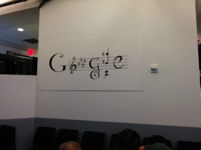
Google I/O Extended NYC

May 19, 2016May 19, 2016 ~ Athar

googleiowelcome

Yesterday I attended the Google I/O Extended event at Google NYC. I used to work there prior to graduate school, so it was great to be back there. I got to see some interesting tech talks, meet up with old friends from Google, and watch a live stream of the keynote.

When I got there, they had coffee and breakfast for everyone, so I happily helped myself to some while checking out the swag they gave us and snapping some pictures:

google_sign1 — I always loved the Google signs in their offices

The stage was of course in Google’s colors

Continue reading →

Enayat Models – ASL 2016

May 16, 2016September 10, 2016 ~ Athar ~ Leave a comment

diagram_transparent

I will be contributing a session at the ASL 2016 North American Annual Meeting, on Wednesday, May 25 at 4:45 PM.

Abstract: Simpson used arithmetic forcing to show that every countable model $\mathcal{M} \models \textsf{PA}$ has an expansion $(\mathcal{M}, X) \models \textsf{PA}^*$ that is pointwise definable. The natural question then is whether this method can be used to obtain expansions of (countable models) with the property that the definable elements of the expansion coincide with the definable elements of the original model. Enayat later showed that this is impossible. He proved that there are models with the property that every expansion upon adding a predicate for an undefinable class is pointwise definable. We call models with this property Enayat models. It is easy to iterate Enayat’s construction and obtain other models with this property. Elementary submodels of any Enayat model formed in this way are well-ordered by inclusion. I will present a construction of an Enayat model whose elementary substructures form an infinite descending chain.

Slides from this talk.

Pi5NY Math Competition

May 9, 2016May 17, 2016 ~ Athar ~ Leave a comment

This past weekend, I had the opportunity to volunteer at the AMS Pi5NY Math Tournament. This tournament is held annually, open to middle schoolers in any of the 5 boroughs of NYC.

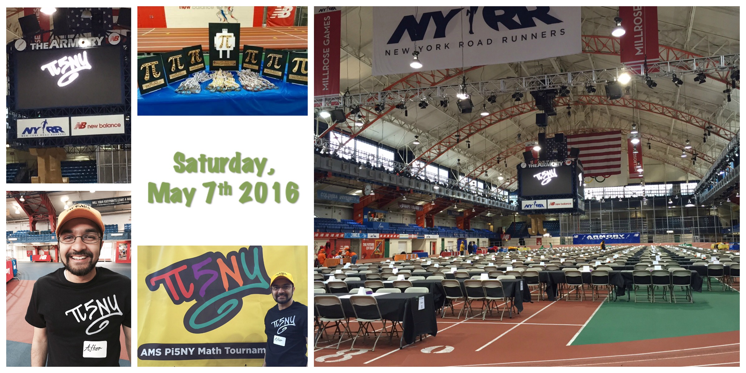
Students worked in teams of 5 on a set of 40 problems. I was a judge for two 8th grade teams. When one of the students finished a problem, they would come to me and I would check their answer, and then send them off to the scorers if their answers were correct.

It was a lot of fun and great to see so many young people enjoying math on a Saturday morning!

Athar Abdul-Quader

Mathematical Logic / Models of Arithmetic