In this post, I will go through a proof of one of my favorite results in combinatorics using a technique that is not necessarily well known outside of logic.

Ramsey’s Theorem

There are many ways to describe (Infinite) Ramsey’s Theorem. One description uses graph theory. A graph is a set of vertices (nodes) and edges (connections between the nodes). A clique in a graph is a subset X of the set of vertices such that all vertices in X have edges between them. An anti-clique is a subset X of the set of vertices such that no two vertices in X have edges between them.

Theorem: Every infinite graph has an infinite clique or an infinite anti-clique.

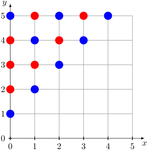
We can formalize Ramsey’s Theorem in another way. A two-coloring of a set X is a function $f : X \to \{ 0, 1 \}$ ; in other words, a partition of X into two sets (the elements 0 and 1 are the “colors”, often representing blue and red). GIven a set X, the set $[X]^2$ is the set of pairs of elements of X. For example, the set $[\mathbb{N}]^2$ is the set of (unordered) pairs of natural numbers, e.g., it’s the set {0, 1}, {0, 2}, {1, 2}, {0, 3}, etc.

Theorem (Ramsey’s Theorem for Pairs): If f is a two-coloring of $[\mathbb{N}]^2$ , there is an infinite set H such that all pairs of elements of H get the same color.

These two theorems are equivalent: given a two-coloring of the set of pairs of natural numbers, you can form an infinite graph by letting the set of vertices just be $\mathbb{N}$ , and by putting an edge between numbers n and m if and only if the color $f(n, m) = 1$ . You can also go the other way: given a graph, you can form a two-coloring of the set of pairs of vertices of the graph in a canonical way.

This second statement, while more difficult to parse, is the one we will focus on for this post.

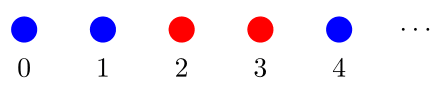
First, let’s prove an easier statement: if $f$ is a two-coloring of $\mathbb{N}$ , there is an infinite set X such that every element of X gets the same color. (This would be referred to as “Ramsey’s Theorem for Singletons”.)

ramsey-1 — A two-coloring of $\mathbb{N}$

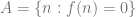
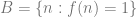
This result is fairly easy to prove: let $A = \{ n : f(n) = 0 \}$ and $B = \{ n : f(n) = 1 \}$ . One of these two sets must be infinite, and every element of A gets color 0 (blue), while every element of B gets 1 (red).

If we try to generalize this proof to Ramsey’s Theorem for Pairs, we can look at the sets $A = \{ \{ x, y \} : f(x, y) = 0 \}$ and $B = \{ \{ x, y \} : f(x, y) = 1 \}$ ; clearly one of these is infinite. But these sets are sets of pairs, and Ramsey’s Theorem states that there is an infinite set of numbers where all the pairs of numbers get the same color (in graph-theoretic terms, it’s easy to find an infinite set of edges or non-edges in an infinite graph; we want an infinite set of vertices which are either all mutually connected or mutually disconnected).

The reason Ramsey’s Theorem for Singletons is easy to prove is because we know the color of each number; we know $f(0), f(1),$ etc. But if we are coloring pairs, then perhaps $f(0, 1) = 0, f(0, 2) = 1, f(0, 3) = 0,$ . In other words, the color of 0 might be blue infinitely often, and it might be red infinitely often. We need a way to decide the color of each natural number “on average”. That is, if we could say, given a natural number n, “for most numbers m, $f(n, m) = 0$ “, or, “for most numbers m, $f(n, m) = 1$ “.

Of course, it is not obvious that it is possible to make such a claim for each number n. Sometimes it’s clear: if, for example, the color “stabilizes”; ie, maybe $f(0, 1) = 0, f(0, 2) = 1, f(0, 3) = 0,$ and for all $n > 3$ , $f(0, n) = 1$ . In that case, it is clear that the color of 0 is “usually” 1. But perhaps the color does not stabilize: maybe there are infinitely many numbers m such that $f(0, m) = 0$ and infinitely many n such that $f(0, n) = 1$ . So in that case, how would you decide what the color of 0 is on average?

Ultrafilters: “averaging” over infinity

This idea of averaging over an infinite set can be studied formally with the concept of an ultrafilter. An ultrafilter is a way of choosing which sets are “large”.

Definition: A filter on the natural numbers is a family of sets $\mathcal{F}$ with the following properties:

for any sets A and B, if $A \in \mathcal{F}$ and $A \subseteq B \subseteq \mathbb{N}$ , then $B \in \mathcal{F}$
for any sets $A, B \in \mathcal{F}$ , the intersection $A \cap B \in \mathcal{F}$
$\emptyset \not \in \mathcal{F}$ .

An ultrafilter is a filter $\mathcal{U}$ with the additional property that for all $X \subseteq \mathbb{N}$ , either $X \in \mathcal{U}$ or $\mathbb{N} \setminus X \in \mathcal{U}$ .

Again, the idea is that the sets in an ultrafilter are considered “large”. Each of these properties represents some “largeness” principle. If a set is large, any set that contains it should also be large; if two sets are large, their intersection is large; the empty set is not large; and if a set is not large, the complement of it should be large. We say that a property “almost always” happens if it happens on a large set, and it “almost never” happens if it happens on a set which is not large.

There are some easy examples of ultrafilters: take any number n, and let $\mathcal{U}_n = \{ A \subseteq \mathbb{N} : n \in A \}$ . It’s not hard to verify that all the properties are satisfied. Ultrafilters like these (the ones generated in some sense by a single number) are called principal. Non-principal ultrafilters are harder to construct, but given some amount of set theory it is possible to show that they also exist. Non-principal ultrafilters have a crucial property: they contain no finite sets. That means that if A is the complement of a finite set (“cofinite”), then A is in every non-principal ultrafilter.

Proof of Ramsey’s Theorem

Let $f : [\mathbb{N}]^2 -> \{0, 1\}$ . Let $\mathcal{U}$ be a non-principal ultrafilter. We use the ultrafilter $\mathcal{U}$ to assign colors to each number as follows: $g : \mathbb{N} \to \{ 0, 1 \}$ is defined as $g(n) = 0$ if and only if $\{ x : f(n, x) = 0 \} \in \mathcal{U}$ , and $g(n) = 1$ otherwise. Notice that $g(n) = 1$ if and only if $\{ x : f(n, x) = 1 \} \in \mathcal{U}$ . In other words, think of $f$ as assigning an infinite sequence of colors to $n$ . Then, using the ultrafilter, we pick out the color of $n$ “almost always”, and call that color $g(n)$ .

We will define a sequence by induction. Let $a_0 = 0$ . Given $a_0, \ldots, a_n$ , let $a_{n+1}$ be the least $a > a_n$ such that $f(a_i, a) = g(a_i)$ for each $i \leq n$ . We must show that such an $a$ exists. The idea here is that the function $g$ assigns the “correct” color according to the ultrafilter; that is, for each $i$ , the set of those $x$ such that $f(a_i, x) = g(a_i)$ is large. Since the intersection of finitely many large sets is also large, the set $X = \{ x : f(a_i, x) = g(a_i)$ for all $i \leq n \}$ is large. Furthermore, in a non-principal ultrafilter, large sets are always infinite, so there must be an $a \in X$ greater than $a_n$ .

Let $Y = \{ a_n : n \in \mathbb{N} \}$ , $B = \{ a \in Y: g(a) = 0 \}$ and $R = \{ a \in Y : g(a) = 1 \}$ . Clearly $Y$ is infinite, so one of $B$ or $R$ is infinite. Further, for all $x < y \in B, f(x, y) = 0$ and for all $x < y \in R, f(x, y) = 1$ , so one of $B$ or $R$ is the infinite set required by the statement of Ramsey’s Theorem.

Other applications of ultrafilters

Ultrafilters have applications all throughout mathematics, including in model theory, social choice, and non-standard analysis. I hope to explore non-standard analysis, in particular, in a future post, where I will discuss ideas like formalizing the notion of a limit using infinitesimals (instead of using epsilons and deltas).

I will be speaking at the Models of Peano Arithmetic seminar on Wednesday, September 21, 2016 on “Ramsey Quantifiers”. The abstract is listed on the NYLogic site, but for context I wanted to provide some thoughts on why I am digging up this older topic.

This theory piqued my interest while I was studying the lattice problem for models of PA. In studying this problem, it became apparent that certain combinatorial properties of representations of lattices were important. Let me preface this by saying that much of this information is in The Structure of Models of Peano Arithmetic, by Kossak and Schmerl, in Chapter 4 on Substructure Lattices.

A representation of a lattice $L$ on a set $A$ is an injection $\alpha : L \to \textrm{Eq}(A)$ (where Eq(A) is the set of equivalence relations on the set A), such that for each $r, s \in L, \alpha(r \vee s) = \alpha(r) \wedge \alpha(s)$ , $\alpha(0)$ is the trivial relation and $\alpha(1)$ is the discrete relation . Given $\alpha : L \to \textrm{Eq}(A)$ and a set $B \subseteq A$ , the function $\alpha | B$ is defined by $(\alpha | B)(r) = \alpha(r) \cap B^2$ for each $r \in L$ . Two representations of the same lattice, $\alpha : L \to \textrm{Eq}(A), \beta : L \to \textrm{Eq}(B)$ are called isomorphic if there is a bijection $f : A \to B$ respecting the equivalence relations; that is, for each $r \in L$ and $x, y \in A$ , $(x, y) \in \alpha(r) \leftrightarrow (f(x), f(y)) \in \beta(r)$ .

The Lattice $B_2$

The lattice $B_2 = \{0, a, b, 1\}$ is the Boolean Algebra on a 2 element set: (with $0 < a < 1$ and $0 < b < 1$ ). Gaifman proved that every model $\mathcal{M} \models \textsf{PA}$ has an elementary end extension $\mathcal{N}$ such that the interstructure lattice $\textrm{Lt}(\mathcal{N} / \mathcal{M}) = \{ \mathcal{K} : \mathcal{M} \preceq \mathcal{K} \preceq \mathcal{N} \}$ is isomorphic to $B_2$ (in fact, Gaifman’s proof works for every finite Boolean algebra). But we can also form such an elementary extension by studying the appropriate representation of the lattice $B_2$ .

Given a model $\mathcal{M} \models \textsf{PA}$ , there is a particularly simple representation on the set of pairs of elements of $M$ , denoted $[M]^2$ . This representation is defined by letting $\alpha(a)$ be the equivalence relation determined by equality on the first coordinate, and $\alpha(b)$ be the equivalence relation determined by equality on the second coordinate. This representation is definable in $\mathcal{M}$ , by using the normal coding of pairs of numbers (Cantor’s pairing function) and the induced projection functions.

The key lemma we need to construct the elementary extension is that for any definable equivalence relation $\Theta$ on $[\mathcal{M}]^2$ , there is a definable subset $A$ of $[\mathcal{M}]^2$ such that $\Theta \cap A$ is either discrete, trivial, $\alpha(a) \cap A$ or $\alpha(b) \cap A$ , and $\alpha | A \cong \alpha$ . The underlying combinatorics here is a generalization of Ramsey’s theorem for pairs, first proved by Erdős and Rado: given any equivalence relation $\Theta$ on $[\mathcal{M}]^2$ , there is an infinite set $X \subseteq \mathcal{M}$ such that $\Theta \cap [X]^2$ is either discrete, trivial, $\alpha(a) \cap [X]^2$ or $\alpha(b) \cap [X]^2$ . Note that this $X$ is just an infinite set of numbers, not of pairs.

This is similar to the key lemma needed when constructing minimal extensions. If $\mathcal{M}$ is a model, a minimal extension $\mathcal{M} \prec \mathcal{N}$ is an elementary extension such that there are no proper intermediate elementary structures (that is, if $\mathcal{M} \preceq \mathcal{K} \preceq \mathcal{N}$ , then $\mathcal{M} = \mathcal{K}$ or $\mathcal{K} = \mathcal{N}$ ). In that case, we consider any infinite definable set $A$ and show that for any definable equivalence relation $\Theta$ on $A$ , there is an infinite definable $B \subseteq A$ such that that $\Theta \cap B^2$ is either discrete or trivial. The main difference between these two cases is the first order expressibility of these statements. Stating that there is an infinite subset $B \subseteq A$ on which $\Theta$ is discrete or trivial can be expressed in the language of first order arithmetic:

$[\exists x \in A \forall w \exists y \in A (y > w \wedge (x, y) \in \Theta)] \vee [\forall w \exists y > w (y \in A \wedge \forall x < y (x \in A \rightarrow (x, y) \not \in \Theta))]$ .

Even though it appears, at first, we want to say “There is an infinite set” where something holds (which would appear to be a second-order quantifier), we can state this in first order (because by “infinite” we really mean “unbounded”).

In the Erdős-Rado result, something appears to be significantly different, however. We must state: “there is an infinite set $X$ such that either (i) for all $x_1 < x_2, y_1 < y_2 \in X$ , $( (x_1, x_2), (y_1, y_2)) \in \Theta$ , (ii) for all $x_1 < x_2, y_1 < y_2 \in X$ , $( (x_1, x_2), (y_1, y_2)) \in \Theta$ if and only if $x_1 = y_1$ , (iii) for all $x_1 < x_2, y_1 < y_2 \in X$ , $( (x_1, x_2), (y_1, y_2)) \in \Theta$ if and only if $x_2 = y_2$ , or (iv) for all $x_1 < x_2, y_1 < y_2 \in X$ , $( (x_1, x_2), (y_1, y_2)) \in \Theta$ if and only if $(x_1, x_2) = (y_1, y_2)$ . In this case, we cannot replace the second-order quantifier with first order ones asserting unboundedness of some property, because we wish to quantify over pairs of elements from that (unbounded) set.

After thinking about this for awhile, my advisor mentioned a section in Chapter 10 of The Structure of Models of Peano Arithmetic, which discusses an extra quantifier called a “Ramsey quantifier”, denoted $Q^2$ . This quantifier extends the language of first order logic by binding two variables. The intended interpretation of $Q^2 x, y \phi(x, y)$ is “There is an infinite set $X$ such that for all $x \neq y \in X$ , $\phi(x, y)$ holds.” This is exactly the kind of extension to the language that I needed, and I hope to talk about some of the basic results in the theory of Peano Arithmetic in this augmented language (with induction for all formulas in the extended language).